Statistical practice in field epidemiology: so many problems, so many solutions

Some colleagues and I have recently been having an interesting discussion about how we should be taking account of recent statistical criticisms of p values and practices such as stepwise model selection. We work in a field where a lot of statistical analysis is done by non-statisticians, with or without the support of statisticians, often as part of outbreak investigations and sometimes for research projects.

Typical practice in outbreaks is to conduct case-control or cohort studies (depending on the context) to look for associations between putative exposure variables and illness. Typically we begin by examining the relationship of each of our exposure variables with the outcome individually. After that sifting step we typically construct an initial logistic regression model with variables selected using a criterion such as p<0.2, often excluding variables with a possible protective effect.

We then aim to simplify that model by identifying variables to drop (often based on the significance of their estimates) and using likelihood ratio tests to decide. If we are being good we try not to drop any important confounders in this process. When we can’t drop any more variables, we regard that as our final model to be interpreted. Occasionally we might think of possible effect modifiers to include as interaction terms in the model.

I first learned how to do this in Stata (over 20 years ago), and, though I knew the commands to use, I had a fairly superficial understanding of what I was actually doing. Yet at this point I was quite comfortable with what I was doing - this is what we did. Since then I have taken this approach numerous times.

In outbreak investigations we may or may not have prior hypotheses to be tested, and not infrequently we have small sample sizes but a large number of putative exposure variables to be examined. Sometimes our questionnaires have a hierarchy of detail, e.g. we might ask a number of higher-level questions like “did you eat eggs?”, and if the answer is yes, go on to ask more detailed questions about their egg eating or whatever.

Our analytical process may vary. We often don’t have any control over sample size and just have to collect the data that we can. Usually we write some sort of analytical plan in advance of analysis, but what we do may vary according to the amount of data we actually end up with or because of issues with the data. Sometimes we consider alternatives to ordinary logistic regression, such as Firth logistic regression, log-binomial regression, Poisson regression with robust standard errors or exact logistic regression (if we are resorting to exact logistic regression it is usually a sign that things are not going well). Sometimes we will use forward stepwise model selection instead and I know some colleagues have used a combination of forward and backward methods. Sometimes we will try combining explanatory variables or creating new ones, and very occasionally we can end up fitting more than one model.

Interpretation is still very much based on p values and statistical significance. We do look at estimated effect sizes (reasoning that bigger ones are more consistent with a real effect and less likely to reflect residual confounding) and we always present confidence intervals, though they are often wide. Where we do have a prior hypothesis about a particular exposure, we give greater weight to our interpretation of a significant association. You still sometimes see people writing things like: there was “a trend towards significance” for p values that disappointingly don’t quite make the cut, or “there was no association” when we are glad they don’t. And not infrequently we agonise over unexpected statistically significant findings that result from these processes, such as associations between food-borne illness and unlikely causative exposures such as drinking from the water jug on the table or eating the bread rolls (in for example a Salmonella outbreak related to a wedding or funeral). I have seen this type of finding more often ascribed to cross-contamination of foodstuffs than to dodgy statistics.

Rarely are we able to try to replicate our findings in another study, as in many outbreak investigations you only get a single shot at collecting data. But we do try to keep our hypothesis-generating process (such as the in-depth interviews we sometimes do with early cases) distinct from our hypothesis-testing process (as in e.g. a case-control study).

Over the past several years I have deepened my understanding of statistics and started to question some of our conventional practices, as I have realised that they are often pragmatic approaches without any actual theoretical justification. And some of the methods we continue to use have increasingly been criticised in the statistical literature, advised against by learned bodies or even banned by scientific journals.

So do we have a problem?

We can’t really talk about a “replication crisis” in our field as we rarely replicate anything. We are not getting much flak - we are most often engaged in the mundane but worthy task of trying to identify a culprit foodstuff (both as evidence and to guide further investigation), in contrast to the more fanciful stuff based on similar statistical methods that gets published in psychology journals and draws the unwelcome attention of critical statisticians. And old hacks like me take the results of this kind of analysis with a big pinch of salt anyway.

But we should want our findings to be as reliable as possible, as they may have important consequences and can be challenged. Other government agencies can be sceptical about purely epidemiological evidence and courts can regard it as circumstantial evidence.

In my experience, the epidemiological findings of an outbreak investigation are valuable corroborative evidence and useful for guiding other parts of the investigation, such as food sampling and supply network investigation, but often aren’t a “smoking gun” in themselves. For that we still ideally need to demonstrate where the exact strain of bug that caused the illness came from and how it got to the people, which usually requires microbiological and other non-statistical evidence, to be as definitive as it can be.

Unfortunately, by the time the outbreak is recognised and the investigation begins, the microbiological evidence may no longer all be out there. Production turnover can be rapid and food shelf lives can be short. So we do still need the epidemiology to be as good as possible.

The problems with p values have been discussed at length in the scientific and statistical literature. I’ve listed various useful papers on this and related issues here and there may be some more relevant links here.

Basically p values are a flawed criterion for identifying true effects/associations in your data, partly due to the way they are used and (mis)interpreted, and often result in spurious or exaggerated findings. A lot of people don’t realise that even if your result is statistically significant, there can still be a very high probability that your null hypothesis is true, though they do usually realise that statistical significance does not necessarily mean real-world significance. And results that aren’t statistically significant can be ignored or not published or assumed to indicate that there is no association (despite the saying “absence of evidence is not evidence of absence”).

As statistician William Briggs summarises it rather damningly::

“A wee p-value means only one thing: the probability of seeing an ad hoc statistic larger than the one you did see is small given a model you do not believe. This number is as near to useless as any number ever invented, for it tells you nothing about the model you don’t believe, nor does it even whisper anything about the model you do believe. Every use of the p-value, except in the limited sense just mentioned, involves a fallacy.”

This article enumerates over 20 fallacies or misinterpretations related to p values.

I came across this interesting paper defending the p<0.05 approach. I think the argument here is that while p<0.05 is clearly an arbitrary convention, the fact that it has persisted and spread so widely must be evidence of utility. It also argues that the development of scientific knowledge requires conjecture and refutation, claim and counter-claim, and that to make a scientific claim you will often need to come down on yes or no/maybe based on your statistical analysis. You may have to accept getting the wrong answer several times before you get the right (or better) answer. That’s not littering the literature with false-positive studies - that is just how science works. Your p value of 0.04 might just spur someone to do the bigger more conclusive study. I encourage you to read the full paper.

On the other hand this paper examines a range of justifications for significance testing, finding logical flaws in each, and ultimately concluding that use of significance testing “retards the growth of scientific knowledge”.

Stepwise model selection with a backward or forward approach is another issue because it can simply select the most biased or randomly extreme estimates in your data rather than the true effects (particularly if there are no true effects). A model selected in this way also has p values which are difficult or impossible to interpret. Ronald Fisher popularised the use of the p value for simple agricultural experiments at a time when you used a calculator for the trickier parts of your analysis - I wonder what the old grump would have made of what we are doing now.

Our third big issue is that making data analysis decisions as you go along greatly increases the chances of spurious findings - see e.g. “False-Positive Psychology: Undisclosed Flexibility in Data Collection and Analysis Allows Presenting Anything as Significant”. This has been called the “garden of forking paths fallacy”.

A related issue is our use of a hypothesis-testing approach when we don’t have any prior hypotheses, allowing the (signal or noise in our) data to decide which hypotheses are tested (sometimes pejoratively called “data dredging”).

There are other issues with our investigations in that they are observational studies and subject to numerous biases - I won’t discuss those further here.

A lot of our current statistical practice is what people were taught. It is a very simple, influential and well-rooted paradigm: if p<0.05 at the end of this process then yes, if not then no (or don’t know for the more sophisticated). This may be all that remains with some people from that introductory statistics course years ago, but even statisticians are using stepwise methods, with a justification that basically seems to be a weary “well, sometimes you have to”.

I don’t know how much non-statistical colleagues perceive our approach to be problematic. And it is not straightforward to present a more robust approach, because there isn’t exactly unanimity in the statistical profession on alternative approaches. The American Statistical Association has taken a cautious joint position (at least on p values):

• Principle 1: P-values can indicate how incompatible the data are with a specified statistical model.
• Principle 2: P-values do not measure the probability that the studied hypothesis is true, or the probability that the data were produced by random chance alone.
• Principle 3: Scientific conclusions and business or policy decisions should not be based only on whether a P-value passes a specific threshold.
• Principle 4: Proper inference requires full reporting and transparency.
• Principle 5: A P-value, or statistical significance, does not measure the size of an effect or the importance of a result.
• Principle 6: By itself, a P-value does not provide a good measure of evidence regarding a model or hypothesis.

As far as I can see the Royal Statistical Society has not taken a formal written position. The ASA principles mainly address what p values are and are not and call for cautious interpretation with transparency about methods. It is far from a ringing endorsement of p values, but they don’t give a clear message about whether we should continue to use them, or do something else instead or as well.

A colleague asked me recently what other colleagues in our field should take from all this - do we need to change our practice? It seemed inadequate to simply say that people should understand what they are doing better - we have heard similar exhortations for decades without seeing decisive change. What should we do about the dodgy things like stepwise methods? We do need to show people practical alternatives. Does an inference process even exist that can be relied on in inexpert hands to produce robust results?

Should we all become Bayesians? Over the years I have given a few talks on Bayesian statistics to colleagues, partly motivating them by discussions of the problems with p values. I hadn’t intended to portray them as simple drop-in replacements for existing methods - unthinking use of Bayesian methods wouldn’t necessarily solve anything. But I do think more work is needed to evaluate possible advantages of Bayesian methods for us and how we might operationalise them in our practice.

Other questions have arisen. How radical should we be? How radical can we be? Can we wean traditional epidemiologists off p values? How would other partners and scientific journals react to changes in our practice? How much training/retraining might this all take?

As part of our discussion and investigations, I have put together a non-exhaustive (and far from mutually exclusive) list of possible alternative approaches that we have considered or seen suggested as alterations or replacements for our current practice. Some of the related concepts are deeply statistical, but I have tried to keep things simple where possible.

None of the proposed alternatives will necessarily have the appealing apparent simplicity of p values, nor the attractiveness of stepwise regression for those faced with a small data set, a large number of possible causal exposures and/or no prior hypotheses. Some are evolutionary, while some are more revolutionary and might necessitate substantial retraining in my field. Not many of them can be considered to be simple “drop-in” replacements for existing methods. I have tried to order them roughly from least radical to most radical.

Options considered so far:

• We keep doing what we are doing now.

  I mainly include this to show that our current practice is at one end of the range of possibilities - I didn’t come across any recommended approaches that could be regarded as less rigorous than our current practice.

  It could be argued that we are just doing what lots of other people do, and sometimes we have to do it, and if we get wrong answers then that is just the rough and tumble of scientific progress.

• We keep doing what we are doing now but are highly sceptical about our results.

  This is probably where I am now, regarding unexpected results as highly likely to be spurious in the absence of other evidence.

• We keep doing most of what we are doing now but try to adhere to the ASA principles.

  Look at the ASA principles again. They are basically saying that your p value does not tell you much, and almost certainly not what you want it to tell you.

  They have been rephrased here as a list of don’ts:

  • Don’t base your conclusions solely on whether an association or effect was found to be “statistically significant” (i.e., the p-value passed some arbitrary threshold such as p < 0.05).
  • Don’t believe that an association or effect exists just because it was statistically significant.
  • Don’t believe that an association or effect is absent just because it was not statistically significant.
  • Don’t believe that your p-value gives the probability that chance alone produced the observed association or effect or the probability that your test hypothesis is true.
  • Don’t conclude anything about scientific or practical importance based on statistical significance (or lack thereof).

  These are all entirely justified; however they just seem a bit like negging your analysis but not really giving you a more robust alternative.

• We continue to use p values, but improve our use and interpretation, while broadening our statistical toolbox and improving the research questions we ask.

  As described in the paper “The Practical Alternative to the p Value Is the Correctly Used p Value”, we could decide that classic null hypothesis testing is not the be-all and and end-all of statistics and work on improving our research questions, still using p values where appropriate but improving our use and understanding of them.

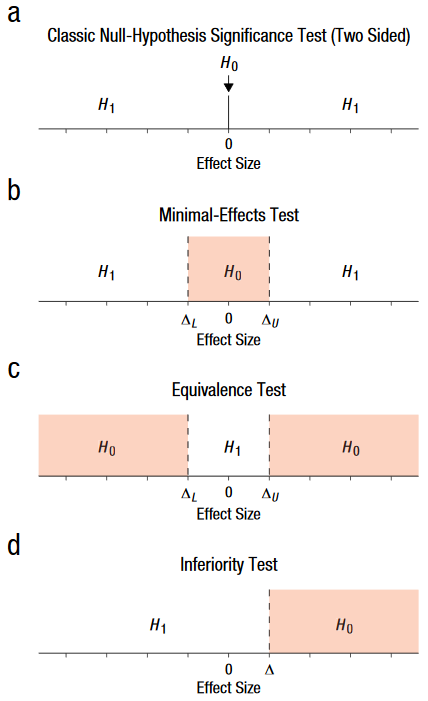
  It is difficult to argue with the proposition that we should do things better. We could review the questions we ask - for example, I doubt the question that the epidemiologist really wants to ask is “is the odds ratio exactly one with infinite precision or absolutely any other conceivable value?”, which is what our current statistical approach is assessing. We could use interval hypothesis tests or minimal effect tests instead.

  

  We might not want to merely know the compatibility of our data with the null hypothesis - we might want to know the probability of our actual hypothesis. We could stop “mindlessly” (sic) applying hypothesis tests. We could consider other analytical approaches - to some extent I am already doing that here.

  It seems implicit in this paper that some of the criticism of p values and the seeking of alternatives is overplayed - p values are not the only game in town, but sometimes they can be appropriate, in which case you should use them right. The famous epidemiologist/statistician Sander Greenland also points out here that some criticisms of p values are not issues inherent to p values and are more related to misuse or misinterpretation.

  To take this more considered approach we would need to raise the level of understanding by our practitioners and (ideally) their audience. Note that the author of the “Practical Alternative” paper has also done a number of interesting massive open online courses (MOOCs) such as this one. Some related materials are here.

• We redefine “statistical significance”.

  It has been argued that using p<0.005 as our new threshold would reduce non-replicability of new research findings in psychology and economics, perhaps by half (note that not all non-replicability of research can be blamed on p values - some is due to other issues such as poor study design). p<0.001 has also been suggested as a new critical threshold for decision-making.

  This would be a fairly simple one to implement but wouldn’t necessarily address issues such as misinterpretation of non-significant results. And in the null hypothesis-testing framework it would presumably increase the probability of type II errors.

• We continue to report p values but not in relation to any arbitrary threshold and stop using terminology that is based on the concept of a critical threshold, including “statistical significance”, “power”, etc.

  This approach is recommended in Rewriting results sections in the language of evidence. According to this paper we should avoid binary language when interpreting continuous p values, such as “statistically significant” (or not), moving closer to how p values were originally used.

  p values were originally devised as a numeric measure of compatibility of the data with the null hypothesis, without any implication of a particular threshold. The origin of p=0.05 as the critical threshold is a bit obscure but it is usually attributed to Ronald Fisher, who later clarified that he regarded p<0.05 as very weak evidence (“significance” meaning to him that it was merely worthy of further attention, not conclusive), and in later life he disavowed the very idea of always using a set threshold.

  Neyman and Pearson took the p value and p<0.05 and built the machinery around it that we use/misuse today to reject the null hypothesis or not, introducing related concepts such as power or type I/II errors. The authors of the “language of evidence” paper recommend a modification of this approach to move away from binary interpretations towards a more continuous/loosely categorical interpretation as shown in the picture below:

  

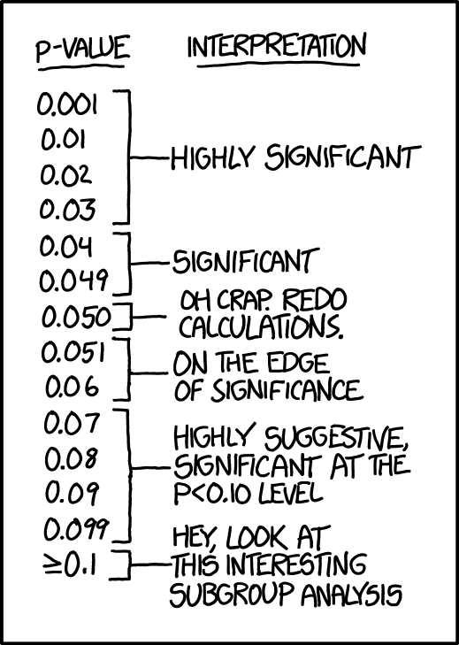
  This is somewhat reminiscent of the famous XKCD cartoon:

  

  There have been various objections to this approach, such as whether p values can really be regarded as evidence. Basically, if the null hypothesis is true then the p value is just a random number, with small values just as likely as large values.

  But you could argue that sometimes you may well need a threshold/decision rule to get an approximate yes/no/maybe answer from your analysis.

• We continue to report p values but focus our interpretation mainly on the estimated effect sizes and their confidence intervals.

  Confidence intervals give more information and we’ve been encouraged to present them routinely for a long time; however this hasn’t necessarily changed our over-reliance on p values.

  This paper recommending an approach dubbed “The New Statistics” provides guidelines (for psychological research, but just as applicable to us), including:

  • Whenever possible, adopt estimation thinking and avoid dichotomous thinking.
  • Do not trust any p value.
  • Whenever possible, avoid using statistical significance or p values; simply omit any mention of null-hypothesis significance testing (NHST).
  • Move beyond NHST and use the most appropriate methods, whether estimation or other approaches.
  • Use knowledgeable judgment in context to interpret observed effect sizes (ESs).
  • Interpret your single confidence interval (CI), but bear in mind the dance. Your 95% CI just might be one of the 5% that miss.

  This brings together a number of ideas already mentioned, e.g.: use the proper tool for the job (you haven’t only got a hammer in your toolbox); if your only evidence is a p value then you may not have much or any evidence at all.

  It emphasises an estimation approach over null hypothesis testing where possible, i.e. base your interpretation on your estimated effect sizes (e.g. odds ratios) and confidence intervals. Would it improve our typical question to change it from “is there evidence consistent with causality by this exposure or not?” to “what are our best estimates of the possible effect/range of effects of this exposure from our data?”?

  Possibly, at least in some scenarios. But confidence interval estimation does share some of the same issues as p values. And I suspect that for some people, their interpretation of the confidence interval may only go as far as “does it include the null value?”, which wouldn’t really move us on beyond the issues of p values.

  A more thoughtful interpretation would be to consider the estimated effect size (we already look to see if it is “large” - perhaps we could pre-specify what is considered big enough) and then examine the range of effects included in the confidence interval to see if they include trivial values (not just the null). Then if we need a decision rule we could have a principled approach of basing our “yes” inferences on estimated effects that are big (enough), precise and inconsistent with trivial effects (in combination with consideration of the context and other evidence), rather than the lottery of p values. We could even routinely plot our confidence intervals to aid this kind of inference. A more nuanced approach to inconclusive results which don’t quite meet those criteria would also be feasible.

  This sort of approach gets us closer to another approach called “Magnitude Based Inference”, where you ignore the null value in your interpretation of the confidence interval, but instead define two other limits which define the range of effects thought to be trivial. This would allow you to interpret a confidence interval in the ways shown in the diagram:

  

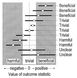
  Magnitude-based inference (MBI) could be an improvement on our practice, and it has been widely used in sports science. It has been presented as the sort of procedure I am looking for, a method that non-statisticians can use without understanding statistics, but with confidence that if they follow the rules they can make valid interpretations and won’t be undermined by devastating critiques of what they are doing in the statistical literature. Unfortunately there are issues with MBI, both theoretical and practical, and there is now at least one devastating statistical critique of MBI.

  It’s been argued that MBI is based on a common subtle misconception of confidence intervals: that the true value has a 95% probability of being in your 95% confidence interval. The 95% probability statement only relates to the procedure in the long run - if I repeat this whole procedure many times then I expect that 95% of all those confidence intervals would include the true value. But the one confidence interval you do have simply either does or does not include the true value. MBI has also been accused of pretending to be Bayesian. There is a true Bayesian version which defines a “region of practical equivalence” (and so the method is called “ROPE”) which is explained here and which may be more robust.

  The practical issue with MBI is that it doesn’t necessarily perform better than null hypothesis testing (in terms of error rates), depending on the limits you chose and the sample size you got. I imagine this might also apply to the Bayesian version.

• We stop using p values altogether and base our interpretation on estimated effect sizes and their confidence intervals.

  This would be a stricter (and perhaps more honest) version of the previous option.

  Not all journals are statistically forward-looking - would they have issues with this? And you can argue that p values are sometimes appropriate.

• We use an alternative statistic to the p value.

  Given the inherent issues with p values, is there a better statistic we can use instead?

  This paper suggests that we use “second generation p values” where our null hypothesis is not just the exact null effect, but also the full range of unimportant effects. This is very similar to the “minimal effect test” idea above.

  S values were proposed by Sander Greenland. An S, or “surprisal”, value is calculated from a p value using the formula $S=-\log_2({p})$. An S value of x means that the probability of your result is the same as the probability of getting all heads when you flip a coin x times (for p=0.05 S is 4.3). While Sander Greenland has probably done more thinking about all these issues than anyone alive, I am not yet convinced that this would be much more intuitive to non-statisticians than p values (except perhaps to coin-based gamblers) or would address all their issues in itself.

• We continue to use p values but adjust them and/or present them with additional information to guide interpretation (of significant and non-significant results).

  We often interpret p values (particularly non-significant ones) in the light of the sample size. Confidence intervals are covered above. But there is other information that could guide more accurate interpretation. It’s been said (only partly in jest) that we should present p values with a range of uncertainty around them.

  This paper recommends “calibration” of p values, but it is not open access so I couldn’t read it.

  Colquhoun (a major critic of p values and not a Bayesian, in case you were thinking that this is all just a pile-on by Bayesians) recommends presenting p values and confidence intervals alongside the false-positive risk (FPR), estimated from your p value and the prior probability of a real effect. He even provides a Shiny app to calculate FPR, though unfortunately only for comparing means.

  Colquhoun thinks that Bayesian methods will never replace frequentist methods, as they not only take account of prior information but must have it, and prior information may be unknown or only subjectively assessed. So he suggests a conservative default of 50% for prior probability of the null hypothesis, for calculation of the FPR (you can play with this assumption in the Shiny app).

  This approach is appealing as it uses the methods we know, and gives you an additional statistic that would be intelligible to non-statisticians.

  Bayes factors could be a useful tool for getting a better quantitative assessment of the evidence our data provides for one hypothesis relative to another, and offer the possibility of using the methods we know but with some additional calculations. A Bayes factor tells you how much more likely your alternative hypothesis (that there is an association) is than your null hypothesis (that there is no association), based on your data. A p value of 0.05 equates to a Bayes factor of around 3 or 4, which indicates that you should update your belief in the probability of the alternative hypothesis by a factor of three or four. Recall that null hypothesis testing only allows you to reject the null hypothesis or not reject it - you can’t say anything about the relative probability of hypotheses. There are conventions (more than one) for the interpretation of the size of Bayes factors, e.g. a BF of >100 could be regarded as “decisive” evidence against the null hypothesis. So it has been suggested that presenting p values alongside Bayes factors could be more informative than presenting p values alone.

  Interpretation of Bayes factors is generally a bit more stringent than that of p values, and as with p values, a more stringent threshold increases the risk of a type II error. Despite the name, they are not a full Bayesian approach. So if your prior belief is that the alternative hypothesis is unlikely, then even a large Bayes Factor might not change your mind. Bayes factors do have subtleties and are not infrequently subject to misinterpretations so would also have training implications. There is a “poke a pizza” explanation of Bayes factors here.

  This interesting paper proposes a kind of reverse Bayesian analysis called “analysis of credibility”: you present your estimated effect size with a confidence interval, then augment this with a “critical prior interval” (CPI) which represents the range of prior beliefs that would be compatible with a Bayesian credible interval (see below) excluding the null effect. For statistically significant results you would only need to calculate the lower bound of the CPI. Interpretation would be as follows: to regard my finding as credible, I would have had to believe prior to the analysis that the true value was contained in the CPI presented. For an example with numbers from the paper: if (in a Salmonella outbreak) my estimated odds ratio for bread rolls was 2.03 and my confidence interval was 1.03-4.00, and the lower bound of the CPI was 10, then I would have had to have expected an odds ratio for bread rolls of at least 10 for my statistically significant finding to be credible. In other words it is not credible.

  This seems attractive as it brings prior information into consideration, while allowing us to use methods we know. It also tackles one of the challenges of going down the full Bayesian analysis route, i.e. “how do I choose my priors?”. But it is clearly a more complex and sophisticated approach which might require substantial retraining of the field epidemiology workforce.

  This paper suggests that doing these three things will solve many p value problems:

  • Redefine statistical significance as p<0.005.
  • Present p values alongside the quantity $\frac{1}{-ep\ln{p}}$, which can be regarded as the upper bound of the Bayes factor, i.e. the alternative hypothesis is at most this times more likely than the null hypothesis.
  • Report your prior odds.

  The first two would be simple to implement; the latter one would require some thinking and possibly some retraining.

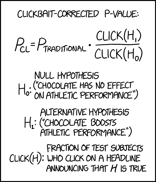
  There are a number of other papers suggesting additional information that can be provided alongside p values, but based on similar ideas such as taking account of prior information. The XKCD cartoon below jokily suggests that we could calibrate our p values against prior information by adjusting for how clickbaity (and therefore unlikely) our findings were.

  

• We continue to use p values but regard them as representing different things depending on how they are being used.

  This seems to be an active area of debate with big names such as Sander Greenland (him again) and Bayesian statistician Andrew Gelman weighing in.

  As a simple example, the p values of exploratory or non-hypothesis driven analysis could be interpreted as having less weight than the p values of a hypothesis-driven analysis. If you follow the links above you will see it can get a little bit more complicated than that.

  This doesn’t yet seem to be a developed enough area for my purposes here.

• We use alternative methods in situations where we don’t have a prior hypothesis.

  If you have a clear hypothesis to test, then you could use a hypothesis-testing approach. If not, then consider alternative methods.

  Penalised regression models (examples are ridge regression, lasso regression and elastic net regression) fit models while penalising for complexity (i.e reducing overfitting). Could these enable a safer approach to stepwise model selection? This presentation by Trevor Hastie seems to suggest so. He describes a scenario that may sound familiar:

  • “In genetic disease studies, we are often faced with modest sample sizes, binary (case-control) responses, and many candidate genes, each a 3-level factor (AA, Aa, aa).”
  • “Logistic regression does not do well in these scenarios: exact aliasing, high-variance coefficients, convergence problems and overfitting.”

  He proposes an R package for stepwise penalised logistic regression model selection (which can do forward or mixed forward/backward selection) called stepPlr.

  This seems promising (though it may be intended for developing predictive models rather than hypothesis testing) but we would need to identify any practical limitations to this approach. I imagine it would not necessarily provide p values that are any easier to interpret, but we could at least partly address this by focussing our interpretation on the effect sizes and confidence intervals.

  Bayesian methods (described below) could also be used as an alternative approach when required. Though Bayesian statistical methods are fundamentally different in several ways from the “frequentist” (based on the expected frequency in a long run of repetitions) statistics you are probably more familiar with, it can be advantageous to take an eclectic approach, using frequentist methods where appropriate and Bayesian methods where appropriate. Some of the ideas above show how taking a Bayesian perspective (particularly in relation to the importance of prior information) when interpreting frequentist results can help you avoid being led into fallacy.

  Prior information can represent either belief or scepticism. Rather than applying our scepticism post hoc and in our heads, we could incorporate it into a Bayesian analysis, which could be useful in the “data dredging, because we have to” scenario. This could have similar benefits for our inferences as the penalised models briefly mentioned above.

• We use Bayesian statistical methods.

  The Bayesian analytical process starts with what you knew before the analysis (expressed as a “prior” probability or probability distribution) and then updates this using your data to give you another (“posterior”) probability or probability distribution. If you have prior information, Bayesian analysis can give you a probability of your hypothesis (with an interval around it representing uncertainty, called a credible interval).

  Bayesian methods are now much more accessible and feasible than before. Not so long ago you might have had to leave clunky Windows software running for hours to fit a Bayesian model - now you can do it in minutes and all in R, Python, Stata or (possibly) your preferred software.

  Another reason that Bayesian methods appeal is that some deep-seated misinterpretations of p values and confidence intervals would be valid interpretations if we were doing a Bayesian analysis. When a non-statistician mistakenly takes a significant p value to mean “the probability I am wrong” or “the probability of the null hypothesis” (things which frequentist statistics can’t give you), then perhaps this represents the questions they really wanted to ask, which Bayesian methods would have been able to answer. With a 95% credible interval, there is actually a 95% probability that the true unknown estimate is in the interval.

  Recall the counter-intuitive mental gymnastics of p values i.e.:

  “If the answer to the opposite of the question we really wanted to ask is yes, and all of our assumptions are correct, the p value is the probability of seeing this test statistic or a more extreme one in either direction in a long run of studies like this.”

  [Food for thought: is “a long run of studies like this” a defensible concept in our applications of p values in (arguably unique) outbreaks where only one sample of data can feasibly be obtained?]

  Wouldn’t epidemiologists prefer to think something along the lines of:

  “If our assumptions are correct, then according to our data the probability of our hypothesis (e.g. that tiramisu is associated with illness) is 75% (95% credible interval 63.3-89.9%).”

  Bayesian modelling allows you to derive other useful probabilities, so you could even think things like:

  “… for this exposure, the probability of an odds ratio greater than 3 (which we regard as the minimally important effect) is 97% (87-100%).”

  Bayesian methods need prior information (which can be quite vague) which is incorporated into the estimation process. This is a double-edged sword. It is useful because (i) it is a Good Thing to take account of what we already know, and (ii) prior information can represent either your belief or your scepticism.

  On the other hand, Bayesian methods can be seen as more “subjective” than frequentist methods. Bayesian reasoning regards probability as your degree of belief in something on a scale of 0 to 1, without any notion of “if you repeated the study many times…”. And different people could come up with different priors, so it is subjective.

  This isn’t necessarily a clear disadvantage compared to frequentist methods. Frequentist analyses often require numerous subjective decisions and are quite undeserving of any label of objectivity. If you don’t believe me, give the same data set and the same research question (with no other instructions) to several different statisticians working independently. It is unlikely that they will all use the exact same methods and get the exact same results. They may have different ways of handling missing data, of recoding their variables, of choosing statistical tests or a multivariable model to fit, etc etc. Some subjectivity is inevitable and it is perhaps just more explicit with Bayesian methods.

  This is not to say that Bayesian statistical methods don’t bring their own complexities. They don’t lend themselves to unskilled use any more than classical statistical methods. Greater use of Bayesian methods would have important training implications. The few talks I have given on Bayesian statistics haven’t so far led to a paradigm shift in field epidemiology, with a grateful workforce rolling out Bayesian statistical methods on a massive scale.

So what do I conclude from all this?

• Firstly, that this really is an area where the more you learn, the less you know!

• Secondly, that our current analytical approach could be improved in a number of areas, but it isn’t just a question of swapping out one set of methods for another, nor is there a better “cookbook” approach out there which we can simply adopt.

• Thirdly, that how we think about statistics needs to develop. This paper, mentioned earlier, puts it better than I could. In brief, we need to “Accept uncertainty” and “be Thoughtful, Open and Modest” (ATOM for short).

  Accepting uncertainty includes “forsaking the false promise of certainty offered by dichotomous declarations of truth or falsity”. Note that the debate about whether we can justify using a threshold value is on-going. But better interpretation of effect sizes and confidence intervals would give us a more sophisticated understanding of our results.

  Being thoughtful means having clear questions, careful study design, appropriate analytical methods, an understanding of what we are doing in the analysis and careful interpretation of your results. Some of this we are already trying to do. For some of our questions, minimal effect tests, penalised regression models or Bayesian methods might be more appropriate.

  p values require very cautious interpretation taking account of context, subject expertise, whether there was prior information, compatibility with other non-statistical evidence, plausibility, what the null and alternative hypotheses were, sample size, power, effect sizes, consideration of what would be considered trivial effects, confidence intervals, other statistics where available, multiplicity (how many hypothesis tests you did - not just the ones you reported…), how closely a pre-specified and detailed analytical protocol was adhered to, how the model was selected and probably other factors too. So simply saying results are “statistically significant” or not will increasingly mark you out as someone who does not know what they are doing. Where we use p values (having considered the alternatives), we should be presenting as much information as we can to aid careful interpretation.

  Being open means transparency in the design, conduct and reporting of your analyses. Share your data, your code and your subjective decisions and be open to external critique.

  Finally, being modest means realising that statistics is just a mathematical thought experiment, using highly simplified conceptual models to represent complex reality. It is not reality and it does not give you truth. I haven’t gone into this here, but sometimes more complex models (e.g. accounting for mediators or colliders) may be more appropriate for causal inference.

• Fourthly, that all of this has training implications. Simply telling people about the issues is no solution for the issues. Introductory statistics courses need to cover a broader “toolbox” of statistical methods, including Bayesian methods, and need to provide a more sophisticated understanding of statistical results. Fortunately such courses are now appearing. Current practitioners may require support through training and statistical support to develop the questions they ask, the range of methods they use and the thoughtful interpretations they make. Journals also have a role to play and may need to adapt.

I think this is my longest post by far! I will try to develop some of the above ideas more practically in future posts.